head(cities) %>% gt() # gt() just makes table look nice :) | names |
|---|
| Bogotá |
| Bogota |
| Québec |
| Quebec |
| Île de la Cité |
| Ile de la Cite |
Below is a collection of R code & tricks I have found helpful to have on hand. These are the smaller, more obscure pieces of code I forget and then repeatedly search online for. I hope to continue to add to this list overtime!
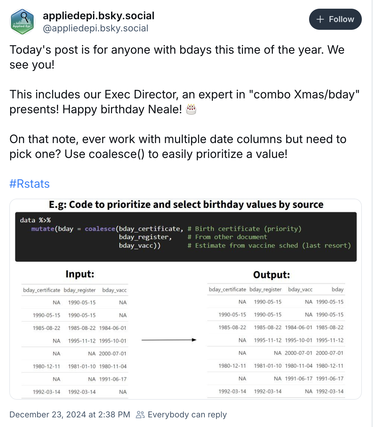
coalesce()Source: post from appliedepi@bsky.social
Returns the first non-missing value from a set of columns based on the order that you specify. This is great for preventing a long series of case_when() calls.
In a situation where we are working with strings with accents (e.g. cities, names, etc), we likely want all strings to be formatted in the same. The following shows an example where some cities have accents and some do not. We can remove all accents using stringi::stri_trans_general(), as shown below.
head(cities) %>% gt() # gt() just makes table look nice :) | names |
|---|
| Bogotá |
| Bogota |
| Québec |
| Quebec |
| Île de la Cité |
| Ile de la Cite |
cities %>%
  mutate(names = stringi::stri_trans_general(names, "Latin-ASCII")) %>%
count(names) %>% gt()| names | n |
|---|---|
| Bogota | 2 |
| Ile de la Cite | 2 |
| Quebec | 2 |
unnest_tokens()The unnest_tokens() is helpful for analyzing word counts of text, specifically that might be split up across many lines. I first used this function to analyze historical markers data. The example below is taken from the unnest_tokens() help page.
library(janeaustenr) # for this example
library(tidytext) # for unnest_tokens()

novel <- tibble(txt = prideprejudice)
head(novel, 15) %>%
gt()| txt |
|---|
| PRIDE AND PREJUDICE |
| By Jane Austen |
| Chapter 1 |
| It is a truth universally acknowledged, that a single man in possession |
| of a good fortune, must be in want of a wife. |
| However little known the feelings or views of such a man may be on his |
| first entering a neighbourhood, this truth is so well fixed in the minds |
| of the surrounding families, that he is considered the rightful property |
novel %>%
  tidytext::unnest_tokens(output = word, input = txt) %>%
  head(20) %>%
gt()| word |
|---|
| pride |
| and |
| prejudice |
| by |
| jane |
| austen |
| chapter |
| 1 |
| it |
| is |
| a |
| truth |
| universally |
| acknowledged |
| that |
| a |
| single |
| man |
| in |
| possession |
We could then go on to count the number of times each word is used!
Like accents, we might also want to remove punctuation. We can do this with the [:punct:] regular expression!
data %>% gt()| feelings |
|---|
| happy :) |
| excited!! |
| **excited** |
| sad :( |
| angry, |
| upset? |
| #mad |
data %>%
  mutate(feelings = str_replace_all(feelings, "[:punct:]", "")) %>%
gt()| feelings |
|---|
| happy |
| excited |
| excited |
| sad |
| angry |
| upset |
| mad |
Many times I have ran into there being a list of words separated by a comma in a column of dataset. For example, asking participants to list the most memorable characteristics of a chocolate that they tasted (analyzed in this tidy tuesday).
This is some code to count how many time each word is used.
head(chocolate) %>% gt()| reviewer | most_memorable_characteristics |
|---|---|
| 2454 | rich cocoa, fatty, bready |
| 2458 | cocoa, vegetal, savory |
| 2454 | cocoa, blackberry, full body |
| 2542 | chewy, off, rubbery |
| 2546 | fatty, earthy, moss, nutty,chalky |
| 2546 | mildly bitter, basic cocoa, fatty |
list_of_adjectives <- chocolate %>%
  mutate(id = row_number(), # gives each reviewer/chocolate combination a unique id
         most_memorable_characteristics = strsplit(as.character(most_memorable_characteristics), ",")) %>% # split on the comma to create a list of characteristics for each individual
  unnest(most_memorable_characteristics) # unlists the list, one in each column

head(list_of_adjectives) %>% gt()| reviewer | most_memorable_characteristics | id |
|---|---|---|
| 2454 | rich cocoa | 1 |
| 2454 | fatty | 1 |
| 2454 | bready | 1 |
| 2458 | cocoa | 2 |
| 2458 | vegetal | 2 |
| 2458 | savory | 2 |
# can then count the number of each adjective, or separate into separate columns:
list_of_adjectives %>%
  group_by(id) %>%
  mutate(adjnum = paste0("adj", row_number(id))) %>%
  ungroup() %>%
  pivot_wider(id_cols = c(reviewer, id), names_from = adjnum, values_from = most_memorable_characteristics) %>%
head() %>% gt()| reviewer | id | adj1 | adj2 | adj3 | adj4 | adj5 |
|---|---|---|---|---|---|---|
| 2454 | 1 | rich cocoa | fatty | bready | NA | NA |
| 2458 | 2 | cocoa | vegetal | savory | NA | NA |
| 2454 | 3 | cocoa | blackberry | full body | NA | NA |
| 2542 | 4 | chewy | off | rubbery | NA | NA |
| 2546 | 5 | fatty | earthy | moss | nutty | chalky |
| 2546 | 6 | mildly bitter | basic cocoa | fatty | NA | NA |
across()across() lets us apply one function to many columns at once, such as below getting the average of each respective penguin measurement column.
library(palmerpenguins)

penguins %>%
  summarise(across(c(bill_length_mm, bill_depth_mm, flipper_length_mm, body_mass_g), ~mean(.x, na.rm=T))) %>%
gt()| bill_length_mm | bill_depth_mm | flipper_length_mm | body_mass_g |
|---|---|---|---|
| 43.92193 | 17.15117 | 200.9152 | 4201.754 |
Use mutate_if() to apply a particular function under certain conditions.
penguins %>%
  mutate_if(is.double, as.integer) %>%  # IF is numeric, make AS integer
  head(3) %>%
gt()| species | island | bill_length_mm | bill_depth_mm | flipper_length_mm | body_mass_g | sex | year |
|---|---|---|---|---|---|---|---|
| Adelie | Torgersen | 39 | 18 | 181 | 3750 | male | 2007 |
| Adelie | Torgersen | 39 | 17 | 186 | 3800 | female | 2007 |
| Adelie | Torgersen | 40 | 18 | 195 | 3250 | female | 2007 |
The data.table package’s fread() function loads data into R more efficiently than many of the read_X() functions. When loading a large dataset, try replacing the read_X() with fread()!
Example of loading in tidy tuesday data:
library(data.table)

historical_markers <- fread('https://raw.githubusercontent.com/rfordatascience/tidytuesday/master/data/2023/2023-07-04/historical_markers.csv')penguins %>%
ggplot(aes(x=flipper_length_mm, y=body_mass_g))+
geom_point()+
labs(x="Flipper length (mm)", y="Body mass (g)", title = "Penguin flipper vs. bill length")+
theme_classic()+
theme(plot.title.position = "plot")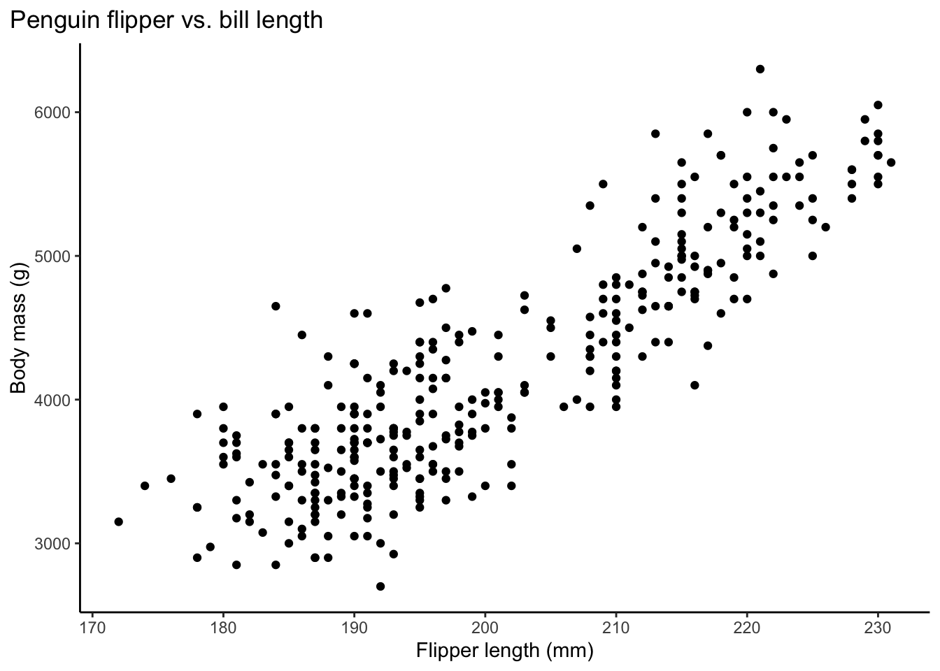
penguins %>%
  ggplot(aes(x=flipper_length_mm, y=body_mass_g))+
  geom_point()+
  labs(x="Flipper length (mm)", y="Body mass (g)", title = "Penguin flipper vs. bill length")+
  theme_classic()+
  theme(plot.title = element_text(hjust = 0.5))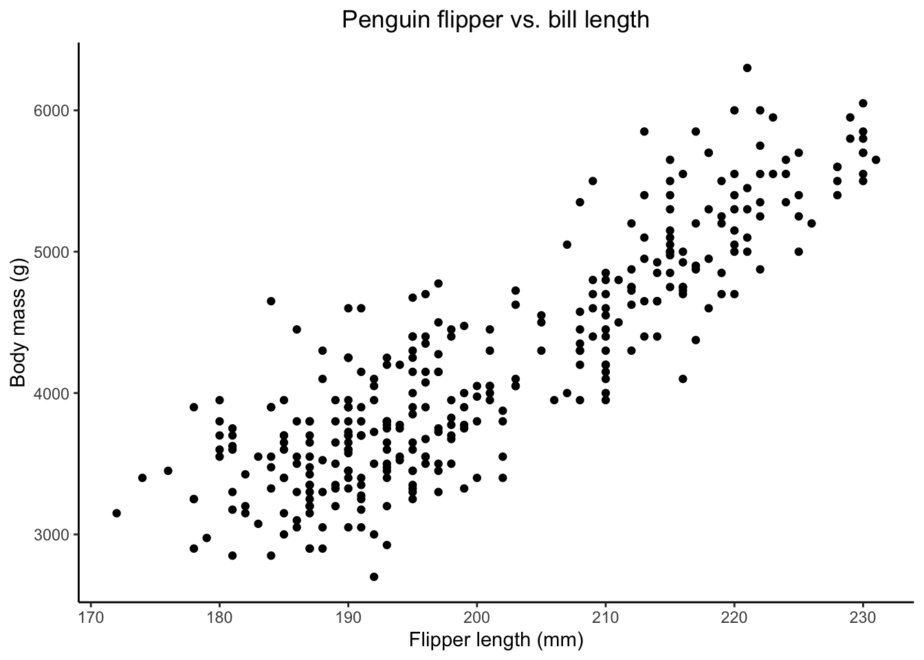
penguins %>%
  ggplot(aes(x=flipper_length_mm, y=body_mass_g))+
  geom_point()+
  labs(x="Flipper length (mm)", y="Body mass (g)",
       title = "Penguin <strong><span style='color:navy'> flipper</span></strong></b> vs. <strong><span style='color:goldenrod3'> bill </span></strong></b>length")+
  theme_classic()+
  theme(plot.title = ggtext::element_markdown()) # must have element_markdown() to make this work!!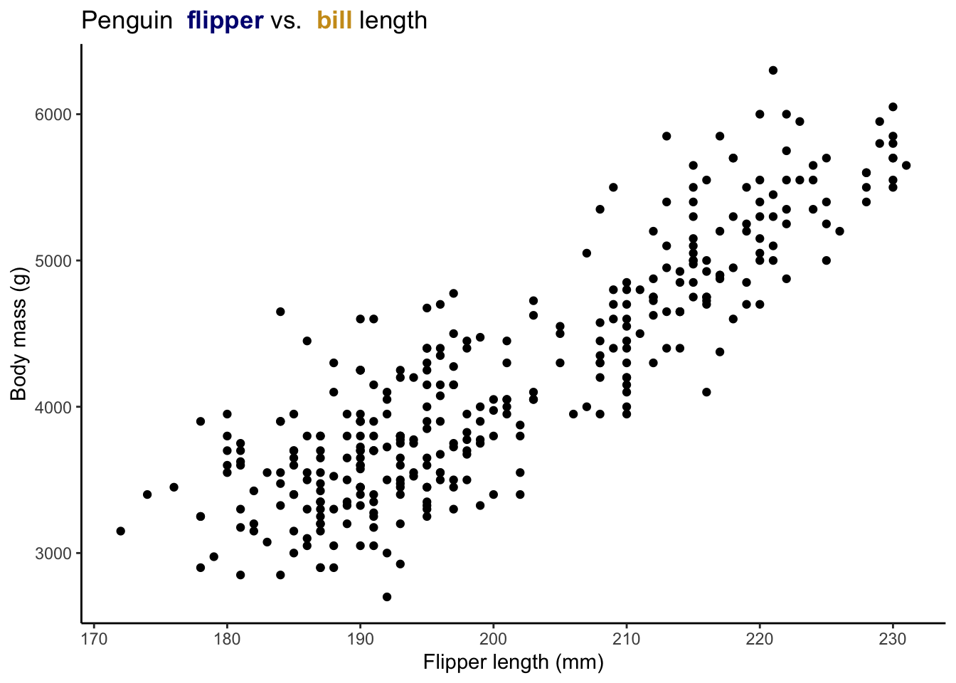
This website is a super fun way to visualize a bunch of different color palettes! You can choose a type (qualitative, diverging, essential), a target color, and the palette length. You can also select for different types of color blindness.
penguins %>%
  ggplot(aes(x=flipper_length_mm, y=body_mass_g))+
  geom_point()+
  labs(x="Flipper length (mm)", y="Body mass (g)", title = "Penguin flipper vs. bill length")+
  theme_classic()+
  theme(plot.background = element_rect(fill = "lightblue3"),
        panel.background = element_rect(fill = "lightblue3"))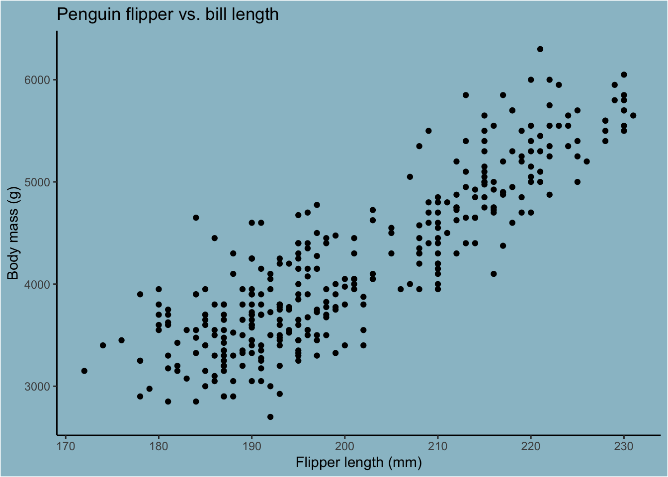
penguins %>%
  ggplot(aes(x=flipper_length_mm, y=body_mass_g))+
  geom_point()+
  labs(x="Flipper length (mm)", y="Body mass (g)", title = "Penguin flipper vs. bill length")+
  annotate(geom="text", x=220, y=3500, label = "There is a \nlinear relationship",
           color = "navy", size=3)+
  theme_classic()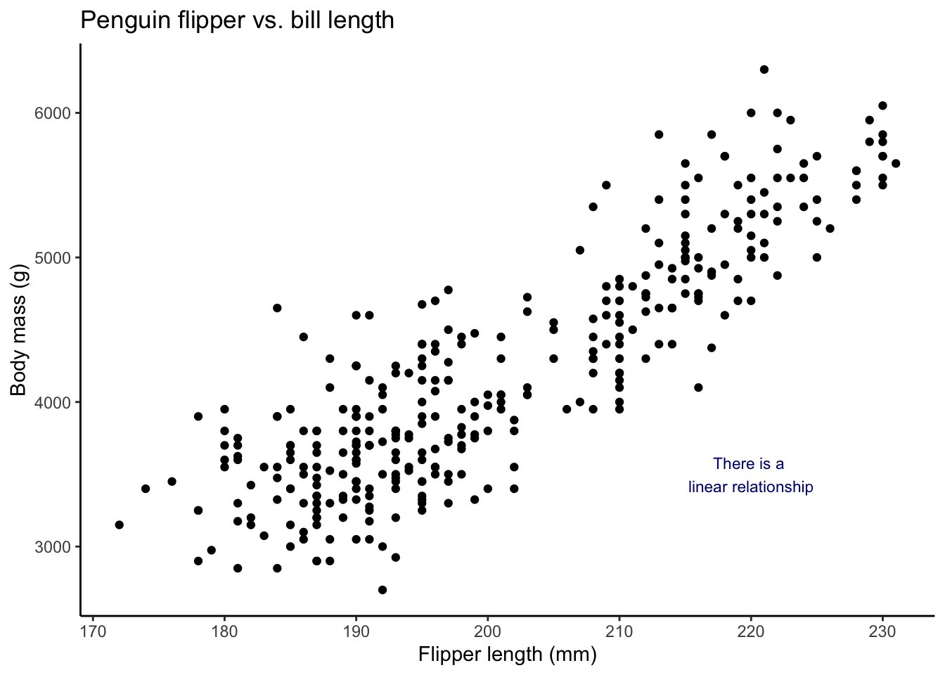
penguins %>%
  ggplot(aes(x=flipper_length_mm, y=body_mass_g))+
  geom_point()+
  labs(x="Flipper length (mm)", y="Body mass (g)", title = "Penguin flipper vs. bill length")+
  geom_curve(aes(x = 220, xend = 211, y = 3500, yend = 4000),arrow = arrow(length = unit(0.03, "npc")), curvature = 0.4, color = "navy")+
  theme_classic()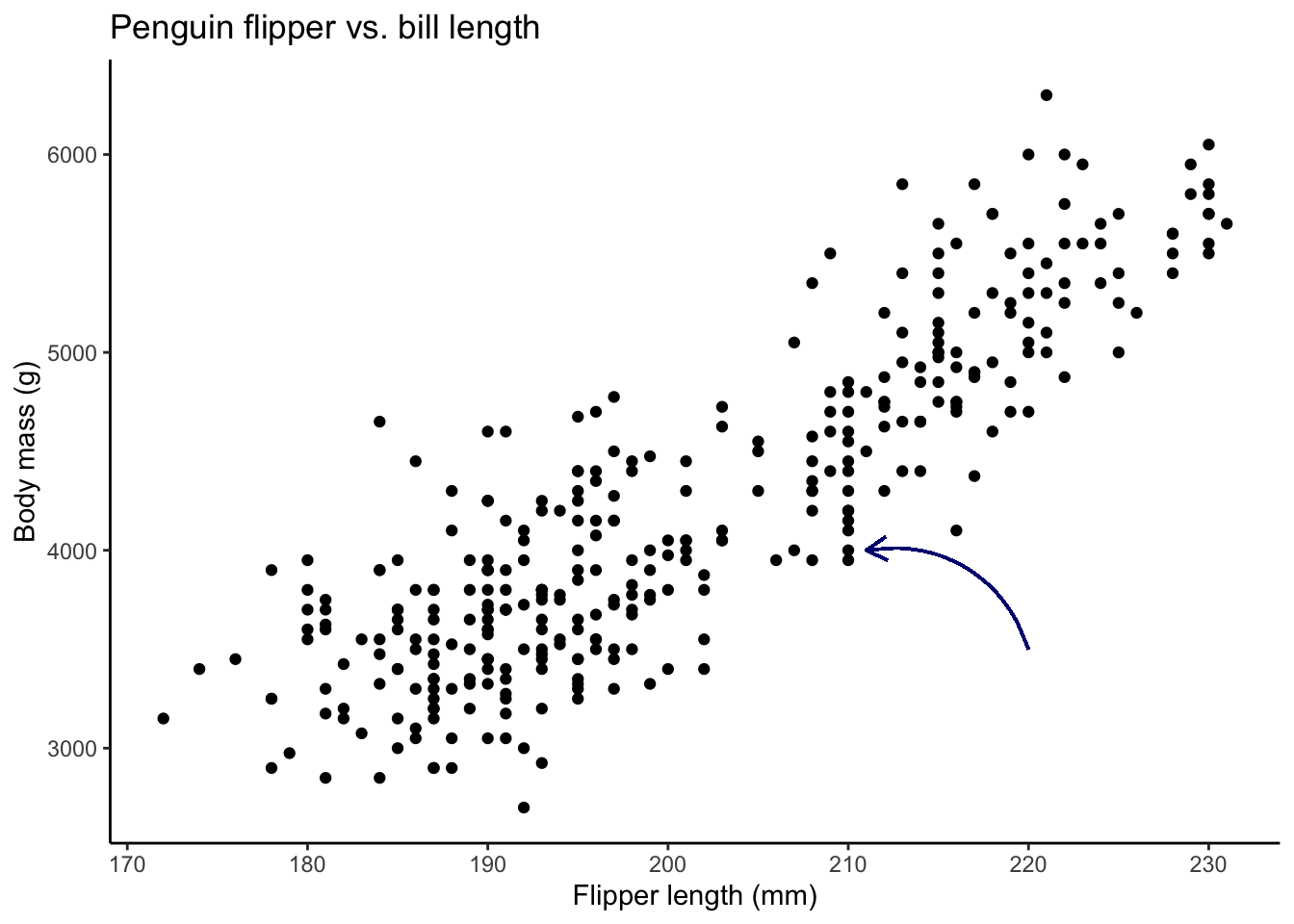
I like the showtext package to change fonts. Look here for fonts.
library(showtext)

font_add_google("Shadows Into Light") # choose fonts to add
font_add_google("Imprima")
font_add_google("Gudea")
showtext_auto() # turns on the automatic use of showtext
penguins %>%
ggplot(aes(x=flipper_length_mm, y=body_mass_g))+
geom_point()+
labs(x="Flipper length (mm)", y="Body mass (g)", title = "Penguin flipper vs. bill length")+
theme_classic()+
theme(plot.title.position = "plot",
plot.title = element_text(family = "Imprima"))
library(png)
penguin_pic <- readPNG("images/penguin.png", native=TRUE)
plot <- penguins %>%
ggplot(aes(x=flipper_length_mm, y=body_mass_g))+
geom_point()+
labs(x="Flipper length (mm)", y="Body mass (g)", title = "Penguin flipper vs. bill length")+
theme_classic()
plot +
patchwork::inset_element(p = penguin_pic,
left = 0.87,
bottom = 0.5,
right = 1,
top = 0.7)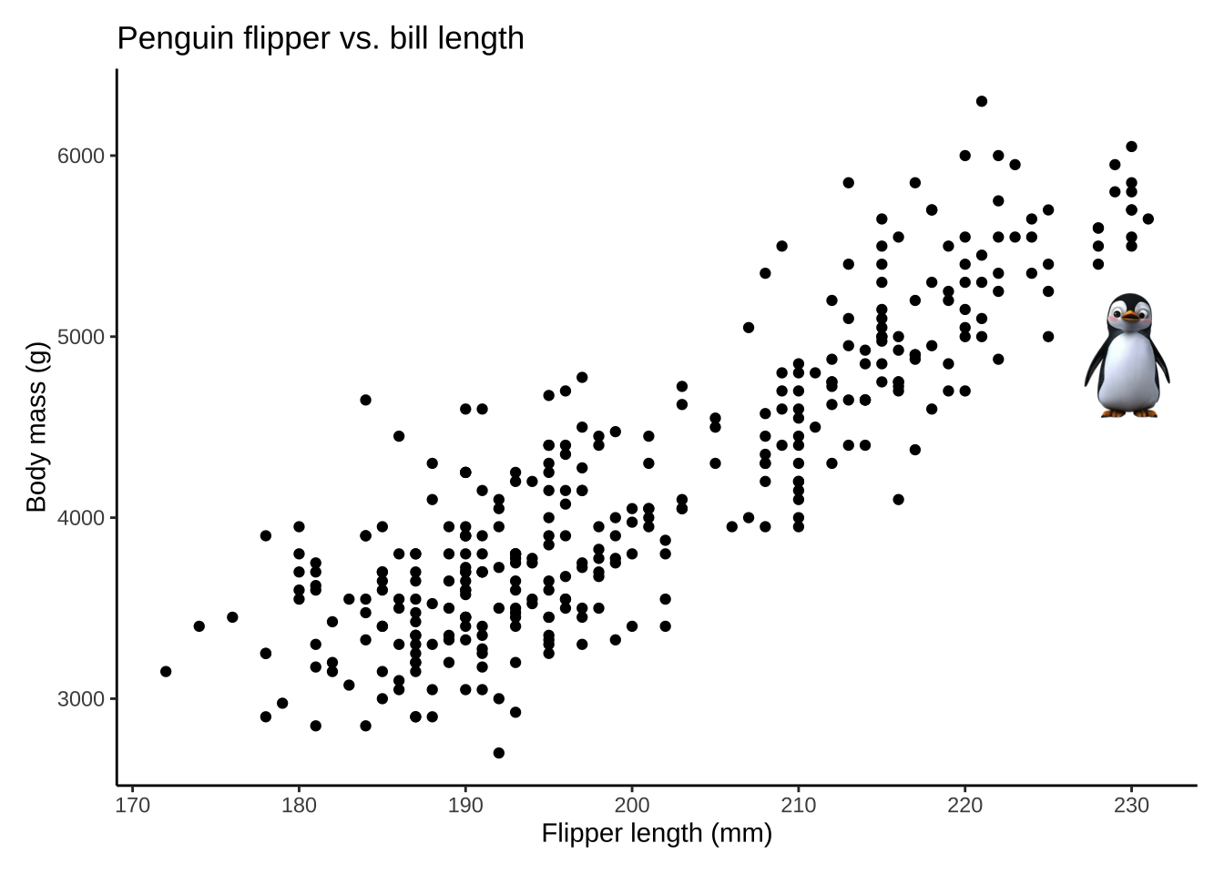
You might not want to do this for a ton of points, but you can replace a typical geom_point() with geom_image(), or think of other fun ways to use this (e.g. putting images at the end of bar chart).
penguins %>%
  head(10) %>% # select 10 points
  mutate(img = "images/penguin.png") %>%
  ggplot()+
  ggimage::geom_image(aes(x = flipper_length_mm, y = body_mass_g, image=img), size=0.06) +
  labs(x="Flipper length (mm)", y="Body mass (g)", title = "Penguin flipper vs. bill length")+
theme_classic() 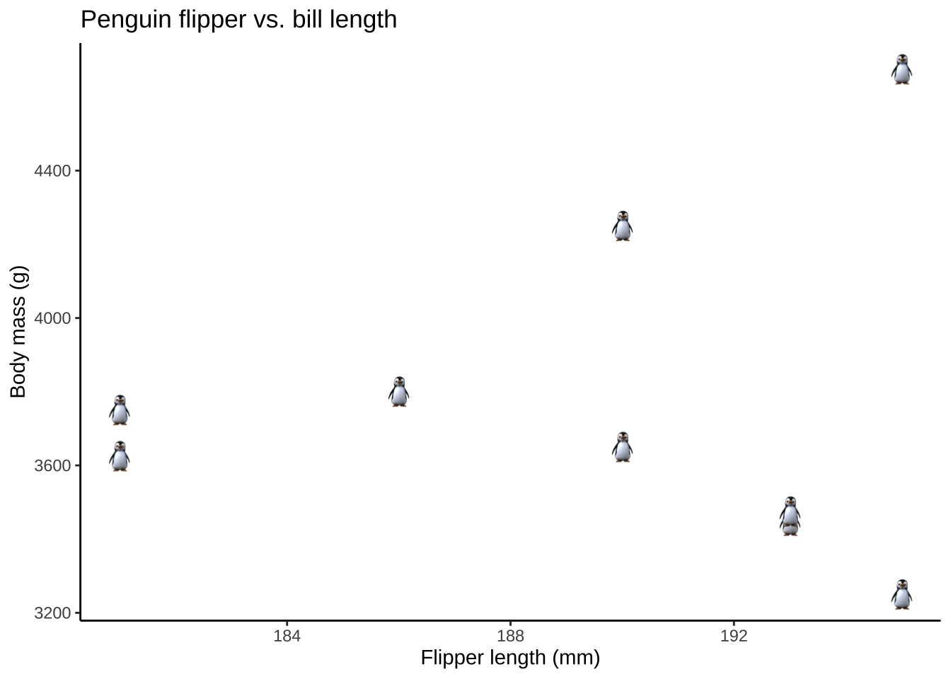
This is super useful for making sure your parentheses are in the right place with a long sequence code!
To turn on rainbow parentheses, go to Tools \(\rightarrow\) Global Options \(\rightarrow\) Code \(\rightarrow\) Display \(\rightarrow\) Use Rainbow Parentheses ☑
During college (and still now) I liked to modify the theme() of a plot a lot. This ended up with a lot of repeated code, so my advisor, Brianna Heggeseth, taught me how to setup a custom default theme. Thanks, Brianna! :) Here are the steps.
Open you .Rprofile file by pasting file.edit(file.path("~", ".Rprofile")) in the console
Modify this file to load your theme when a specific package is loaded (for example, ggplot2). Then, put your desired theme in theme_set(). This could be something as simple as ggplot2::theme_classic(). Below, I put a very simple example of a custom theme.
setHook(packageEvent("ggplot2", "onLoad"),
        function(...) ggplot2::theme_set(ggplot2::theme_classic()+
                                           ggplot2::theme(plot.title.position = "plot",
                                                 plot.title = ggplot2::element_text(family = "mono"))))
A few notes:
- You must call each function you use with the appropriate library in order for this to work.
- When you are done, save the .Rprofile and quit RStudio in order for the changes to be saved.
Here is a source I used to help refresh my memory on doing this.
While making this blog post, I wanted to be able to highlight the lines of code that corresponded to the topic I was discussing. To do this, I installed the line-highlight extension for Quarto and followed the directions.
Thanks for reading my first blog post! If you have any R tricks you know of or feedback on this post, please email me at efranke@andrew.cmu.edu; I’d love to hear :)